In this article I have shown the best 3 methods to insert automatic serial number in MS Excel. These methods will work all the Microsoft version like 2003 to 2021 and Microsoft 365, but before that listen learn how to create table in Excel.
How to Create Table in MS Excel?
Step 1: Select a cell range where you want to create a table, then Go to Insert, and tap on Table button, select the table style from available option.
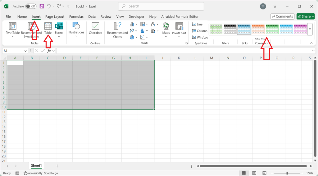
Step 2: Enter your Data into the table. select a location to save your spreadsheet, such as your desktop or documents folder. Name your project file, Select the desired file format, such as “.xlsx” or “.csv “. Choose a location to save your spreadsheet and click “Save.”
How to insert serial number in Ms Excel?
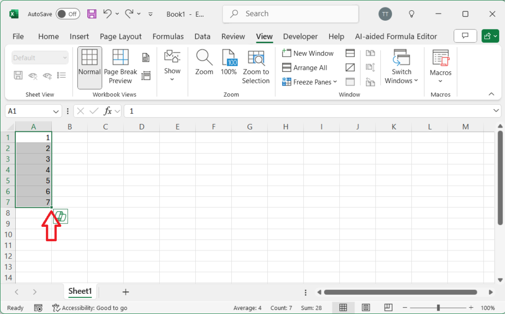
Select the cell where you want to start the serial number, enter the starting number in the selected cell, select the range of cells where you want to insert the serial numbers, drag the fill handle down by holding Ctrl button to fill the range with serial numbers.
How to insert serial number in Ms Excel by using Formula?
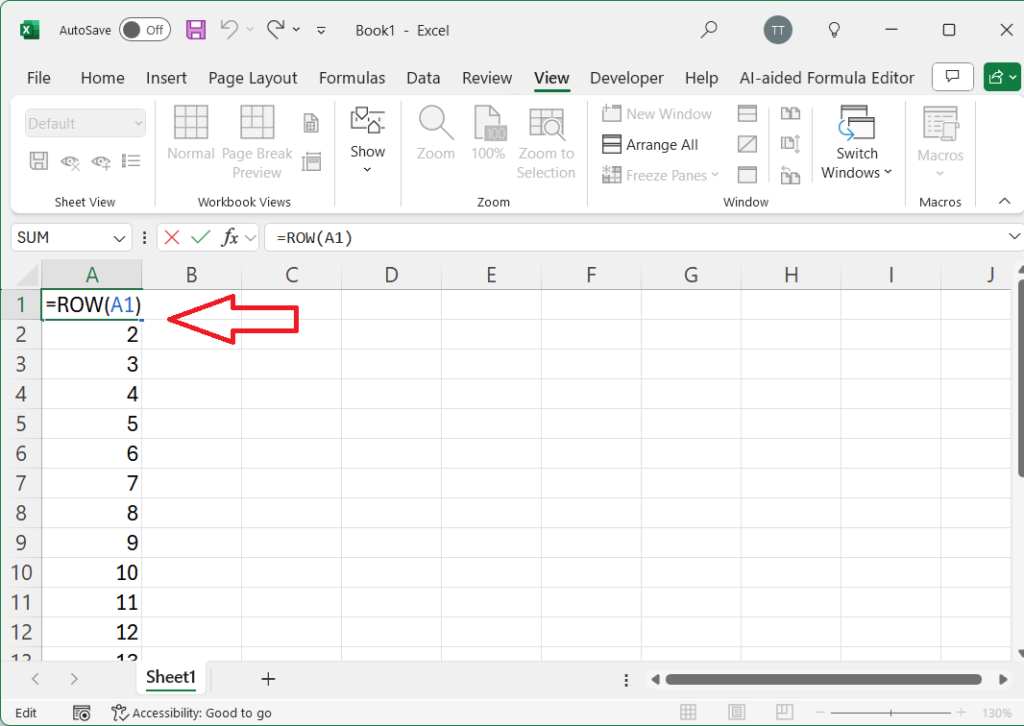
Select the cell where you want to start the serial number enter the formula =ROW(A1) (assuming you want to start from row 1). Copy the formula down to fill the range with serial numbers.
How to insert serial number in Ms Excel by using auto fill feature?
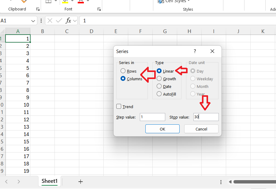
Step1: Select the cell where you want to start the serial number. enter the starting number in the selected cell. Go to the Home tab. click on the Fill & Flash Fill button in the Editing group.
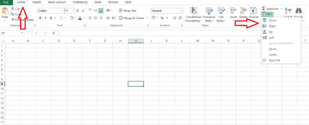
Step 2: A Series will be open, select columns or rows, select Linear, insert your required maximum Number in Stop value then ok
Some Useful Arithmetic Formulas
To find SUM: =SUM(range) Adds up a range of numbers.Example: =SUM(A1:A10)
To Find AVERAGE: =AVERAGE(range) Calculates the average of a range of numbers.Example: =AVERAGE(A1:A10)
To COUNT numbers: =COUNT(range) Counts the number of cells in a range that contain numbers.Example: =COUNT(A1:A10)
To find MAXIMUM VALUE: =MAX(range) Returns the maximum value in a range of numbers.Example: =MAX(A1:A10)
To find MINIMUM VALUE: =MIN(range) Returns the minimum value in a range of numbers.Example: =MIN(A1:A10)
Logical Formulas:
Formula for IF: =IF(logical_test, [value_if_true], [value_if_false]) Tests a condition and returns one value if true and another value if false.Example: =IF(A1>10, “Greater than 10”, “Less than or equal to 10”)
Formula For AND =AND(logical1, [logical2], …) Returns true if all conditions are true.Example: =AND(A1>10, B1<20)
Formula for OR: =OR(logical1, [logical2], …) Returns true if any condition is true.Example: =OR(A1>10, B1<20)
Text Formulas
CONCATENATE: =CONCATENATE(text1, [text2], …) Joins two or more text strings together.Example: =CONCATENATE(A1, ” “, B1)
LOWER: =LOWER(text) Converts text to lowercase. Example: =LOWER(A1)
UPPER: =UPPER(text) Converts text to uppercase. Example: =UPPER(A1)
Date and Time Formulas
TODAY: TODAY() – Returns the current date. Example: =TODAY()
NOW: =NOW() Returns the current date and time. Example: =NOW()
DATEDIF: =DATEDIF(start_date, end_date, unit) Calculates the difference between two dates in a specified unit (days, months, years).Example: =DATEDIF(A1, B1, “D”)
Tips to make professional excel sheet:
- Always use readable font’s style like Times New Roman, Arial, and Calibri etc.
- Always highlight your column headers with bold text or italic.
- Always use formatting like colours, borders, or alignment to make your worksheet more attractive.
- Always data validation to control the input output of your data.